
Technical description
Resolution: 2.05 terapixels, 2 297 216 × 891 702 pixels
Size: 6 TB in uncompressed 8-bit TIFF format.
Multiresolution image pyramid: Total roughly 400 GB.
Built from 366 843 carefully chosen photos (12.3 TB RAW) collected over 4 days from Holmenkollen Ski Tower. The project blends detailed field photography with powerful computational work. Each frame was shot using up to 20 exposures per image, aligned at sub-pixel precision, processed by custom-built software, and finally stitched to deliver a seamless 360° glimpse of Oslo — from fjord to skyline — in unprecedented detail.
About the project
- Scope: 500 000+ captures, 366 843 used in the final panorama.
- Workflow: Median stacking, sub-pixel aligning, optical-flow correction, AI-driven upscaling, multi-threaded GPU rendering.
- Timeline: One year of research/prototyping/building camera rig, four days of capture, one month of image preparation, 2 weeks of RAW development, 2 weeks of intensive processing, 2 weeks of final rendering; and approximately two months of post-processing. Some of the steps repeated several times.
- Infrastructure: Over 50 TB of fast NVMe/RAID scratch storage, 160 TB of archival storage, 100 Gbps networking, and a workstation running dual RTX 4090 GPUs at full load for weeks.
The image
9000 x 4320 desktop
This panorama was edited on 55″ 8K display, but even this was to small and I had to extend the desktop to 9000 x 4320. Note that one and each of the tiny thumbnails represents 180MP image. This part is one of 4 parts which made the whole panorama.
About the technology
1. Preperation
The idea for this project was born after experimenting with CUDA programming and exploring the possibility of performing fast median stacking on the GPU. Confirmation of that CUDA-based median stacking could be executed very fast opened the practical possibility to super-resolution images on a large scale. I decided to take the project further by exploring possibility of photographing from the Holmenkollen Ski Tower.
2. First some theory
2.1 Understanding noise
Originally developed for the Hubble Space Telescope, NASA has developed an algorithm called Drizzle (Variable Pixel Linear Reconstruction) which makes Super Resolution-images by stacking several images. I use Enhanced Correlation Coefficient (ECC) to register (stack on top of eachother) my images, as the Drizzle algorithm do, but there are 2 main differences between my approach and Drizzle approach.
- Drizzle preserves noise (important in astrophotography), while I’m trying to remove noise by applying median stacking.
- Drizzle calculates pixel values by summing and weighting sampled values and then fills the HR (high resolution) grid smoothly, while I map “hard” into the HR grid by applying nearest neighbour upscaling.
ECC is one of the most popular methods for achieving sub-pixel alignment. My approach is robust, median-based upscaling with sharpening afterwards.
Drizzle approach is physically correct reconstruction with weighted pixel spreading (pixfrac), preserving both resolution and noise properties.
Median stacking works like this: For each pixel position across the stack, collect the values of that pixel from all the images. Sort all pixels from darkest to brightest and pick the one in middle.
Key points about considering noise:
1. Noise hides details
- An image = signal (the real scene) + noise (random variation).
- When noise is strong, fine details (thin lines, textures, faint features) get buried under randomness.
- The eye (or algorithms) struggle to separate true detail from random “grain.”
2. Better SNR (signal-to-noise ratio)
- Reducing noise increases the signal-to-noise ratio (SNR).
- Higher SNR means fine structures become clearer.
- This can look like higher resolution, because details that were invisible before become perceptible.
3. Sharpening and resampling work better
- Techniques like unsharp masking, deconvolution, or super-resolution work best on a clean signal.
- If you sharpen a noisy image, you also sharpen the noise = ugly artifacts.
- If noise is reduced first, algorithms can enhance real high-frequency detail without boosting randomness.
4. Theoretical limit
- Noise reduction doesn’t create new information.
- But it gives you better access to the information that was already there, because the noise no longer masks it.
- With multi-frame stacking (median/mean), SNR increases and you can exploit the sensor’s true resolution.
Summary
Noise reduction improves image quality because hidden details emerge from under the noise. It can feel like increased resolution, even though the pixel grid hasn’t changed. When combined with techniques like Drizzle or multi-frame super-resolution, you get both better SNR and a finer sampling grid, which yields genuine resolution gain.
2.2 Understanding digital enhancing of images
Sharpening
Sharpening in digital images works by enhancing the high-frequency components, which correspond to rapid intensity changes such as edges and fine textures. Techniques like unsharp masking or high-pass filtering detect these variations and boost their contrast, making the boundaries between objects appear crisper. The illusion of added clarity comes from the stronger definition at boundaries and textures.
However, sharpening has a natural limit. Since noise is also made up of high-frequency components, strong sharpening will amplify noise along with real detail, leading to a grainy or harsh appearance. Excessive sharpening also introduces artifacts such as halos—unnatural bright or dark outlines around edges—which can be distracting. At some point, the image stops looking natural: textures may become overly harsh, skin tones can turn plasticky, and the overall impression becomes artificial rather than sharp.
In short, sharpening improves visual clarity by boosting edges, but if pushed too far it amplifies unwanted elements as well, making the result look worse instead of better.
Upscaling
Upscaling is the process of increasing the pixel dimensions of an image, essentially creating a larger grid to display the same visual information. Since no new details exist in the original data, the goal of upscaling is to estimate what the missing pixels should look like by interpolating from the known ones. Different interpolation methods achieve this with varying levels of quality.
Lanczos resampling is one of the most respected classical upscaling techniques. It is based on the mathematical sinc function, which has desirable frequency properties and can preserve edges and fine structures more effectively than simpler methods like nearest neighbour, bilinear, or bicubic interpolation. By sampling with a windowed sinc (sine cardinal) kernel, Lanczos produces smoother gradients and sharper edges, giving the upscaled image a clearer and more natural appearance.
Still, like all single-image interpolation methods, Lanczos cannot recreate genuine detail that was absent in the original. It can only infer values that are consistent with the existing pixel structure. This means the image may appear sharper and cleaner after upscaling, but the true resolution—the amount of real-world detail captured—remains the same. The improvement lies in the quality of the interpolation, not in the recovery of new information.
To genuinely increase resolution, you must introduce extra data from somewhere. One approach is to use multiple images of the same scene, slightly shifted or dithered, and combine them through techniques like multi-frame super-resolution or Drizzle integration. These methods exploit sub-pixel differences between frames to reconstruct details that a single image could not provide. Another approach is to use prior knowledge encoded in algorithms. For example, AI-based upscaling (such as convolutional neural networks or GANs) is trained on vast datasets of high- and low-resolution image pairs. The AI learns statistical patterns of textures, edges, and shapes, and can “hallucinate” plausible fine details when enlarging an image.
There is solid math behind why a single image cannot yield more real detail without extra information. In signal processing terms, a low-resolution image y is typically modeled as a blurred, downsampled version of an unknown high-resolution scene x: y=D H x+n where H is optical blur, D is downsampling, and n is noise. Many different high-resolution images x can produce exactly the same y after blur and downsampling. That means the inverse problem is non-unique: from one y alone, you cannot uniquely recover the lost high-frequency content. Interpolation (bilinear, bicubic, Lanczos) can only estimate values consistent with y; it cannot determine which of the many possible x’s is the “true” one.
Summary
Real resolution gain requires either additional measurements (more images), domain-specific models (algorithmic priors), or learned knowledge (AI). Without these sources of extra data, upscaling can only interpolate, never truly create new detail.
3. Practical solution
It is important to know the theoretical background to understand what can be achieved and why the result is genuine.
3.1 Challenges when photographing over long distances
Photographing distant objects with an 800mm lens is difficult due to atmospheric disturbances, which distort images beyond few kilometers. Straight features such as building corners, lamp posts, and signs no longer appear straight and looks distorted. Because of this it is challenging to maintain image quality even with a high-resolution lens. An f-stop of f/11 was chosen after careful consideration. When using the 2x extender with the 400mm f/2.8 lens, the combination has to be stopped down to minimum f/8 to get sharp images (it’s designed like this). F/11 was chosen to get some longer depth of field, even if this means loosing some resolution on objects very far away.
3.2 Methods Used
To achieve the best results many approaches were tested and a combination of algorithms was employed:
- Rough image alignment using image features
- Sub-pixel alignment using Enhanced Correlation Coefficient (ECC)
- Farnebäck Optical Flow
- EDSR TensorFlow (Enhanced Deep Super-Resolution)
Applying a median on sub-pixel aligned images effectively reduces noise and preserves fine details, even recovering straight lines in distant objects. A more advanced approach used here involves creating a master image using the median, and then using optical flow algorithm to align source images to the master. This method restores details in trees and moving objects and improves resolution in distant areas.
Further refinement is achieved using EDSR TensorFlow, which enhances the quality of extremely distant objects. This approach helps distinguish texture from noise, resulting in a more visually pleasing image in areas affected by strong atmospheric disturbances. This method was applied to parts of the picture with great seeing. For areas with average seeing or worse, there was no visible gain from the much faster nearest neighbor upscaling. A key part of sub-pixel alignment is applying an unsharp mask at the end to recover fine details.
3.3 The processing pipeline
The pipeline is the result with the goal of enhancing resolution and producing a visually pleasing image. The process can be summarized by the following points:
- Group the images into 4 large sub-panoramas based on optimal suitability (north, south, east, west).
- Divide the images into groups, with each group dedicated to upscaling and creating a 180MP super-resolution image. Each group was a burst of 20 images captured in about 1 second for each burst.
- Correct colors and remove haze for improved clarity.
- Develop RAW files into 16-bit TIFF format.
- Sort the images within each group by sharpness, discarding the two least sharp images.
- Mask out low contrast areas in images to prevent using for features and ECC.
- Identify features for a rough alignment of the images.
- Use the Enhanced Correlation Coefficient (ECC) method to align the images with sub-pixel precision.
- Compute the median and enhance sharpness to create a master image for optical flow correction.
- Apply optical flow correction on all images in the group using the master image as source to correct atmospheric turbulence.
- 4x upscale of images using Nearest Neighbor or Tensorflow EDSR (Enhanced Deep Residual Network).
- Compute the median of the upscaled images.
- Apply an unsharp mask to restore fine details.
- Merge four panoramas into one single large 360° panorama.
- Merge inn the sky and render the final panorama.
3.4 Upscaling
Classical Pixel Shift Upscaling
The original pixel-shift algorithm is based on the simple nearest-neighbor interpolation. While it works well, the initial result is often quite blurry. The “secret” to this method, however, is that this allows for very aggressive sharpening without introducing artifacts. This results in a high-resolution image with significant clarity. The idea behind this is if you scale down an image and scale it up again, then in a perfect world (which you have if you scale down and scale up the same picture) you could apply strong sharpness and get back almost the same image.
Introduction of AI
The TensorFlow EDSR (Enhanced Deep Residual Network) is a far more advanced upscaling method. Whether AI is preferable to nearest-neighbor interpolation can be debatable. In my opinion, the ultimate quality of the upscale depends largely on the quality of the source material. If the source is a high-quality image with little noise, both methods will produce great results.
Why not just stick to the simple nearest-neighbor algorithm?
When processing images of distant objects, perfect sharpness is often unattainable. We are operating at the theoretical maximum resolution of the camera and lens, but this is a minor issue compared to atmospheric disturbance. In such conditions, sub-pixel alignment becomes difficult; the images are far from sharp and appears to “wobble.”
Nevertheless, we can still recover a significant amount of detail, even if the result is not perfect. If the lighting is good, AI upscaling tends to perform slightly better. The output is less noisy, and the AI can reconstruct certain textures, such as roof tiles or patterns in brick walls. In this particular picture, most people probably wouldn’t notice which part was upscaled using TensorFlow EDSR and which part was upscaled using Nearest Neighbour. My current approach is a test, keeping in mind that even better results could be achieved with AI models specifically trained for this type of imagery. In theory, performance would improve significantly if a model were trained specifically on architectural elements like houses, streets, signs, and lettering.
3.5 Quality categorization by distance.
Some thoughts on observations from the sampled images. The images can be roughly categorized by distance:
Distance upto 1-2km:
Superb quality, very little noise, AI-upscaling has little impact, no problems with haze.
Distance 2-8km:
Still high quality, but due to haze and lighting conditions, parts of image start to suffer from lack of contrast when photographed directly to the sun. AI gives some cleaner images and more details in areas far away, specially if the quality was decent to start with. Median stacking shines in restoring straight lines and optical flow brings back structures in trees/leaves, improves some resolution and improves straight lines.
Distance 8km-20km and beyond:
The distance light has to travel through air is so far that there is no point to sample more images or get even bigger lens. AI upscaling cleans up the image, producing a more pleasant result to the eye. Objects on the horizon photographed towards the sun falls apart and lacks details and contrast. The worst images has so little contrast and visible details that it is not possible to find any features and only few of the 20 samples are used in median stacking which results in much visible noise.
1 cm details at 8 km — why this shouldn’t be possible (but looks like it is)
Please bear in mind that the boats are ~8 km away. The wires on the sailboats are ≈1 cm thick. Seeing 1 cm details at 8 km should impress you, because it’s impossible —so what’s going on?
The left image is a single exposure. The right image is the final result after processing, upscaling, and sharpening. With an 800 mm f/11 lens on a 45 MP full-frame camera at 8 km, the theoretical diffraction-limited resolution is only about 7–10 cm.
Stacking and upscaling seem to reveal 1 cm “wires,” but that’s an optical illusion. The camera isn’t resolving the wire’s true thickness; it’s detecting tiny contrast changes. Even far below the resolution limit, a thin wire can block or scatter a little light and register as a one-pixel-wide dark or bright line. Sub-pixel alignment and upscaling enhance these edges, making the wire appear visible even though its width isn’t actually resolved. A 1 cm object might cover ~25% of a pixel, yet repeated frames, careful alignment, and sharpening can pull out that sub-pixel contrast—this image is a good example.
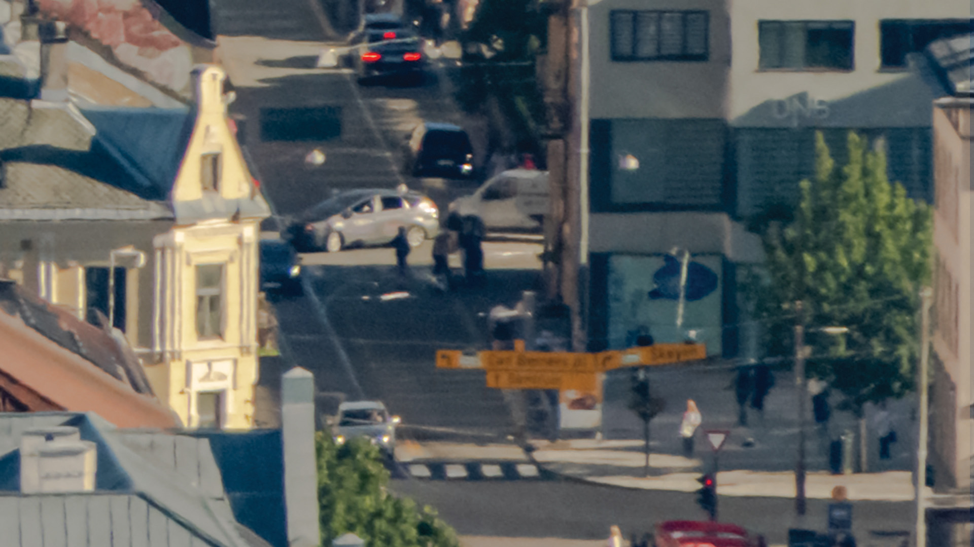
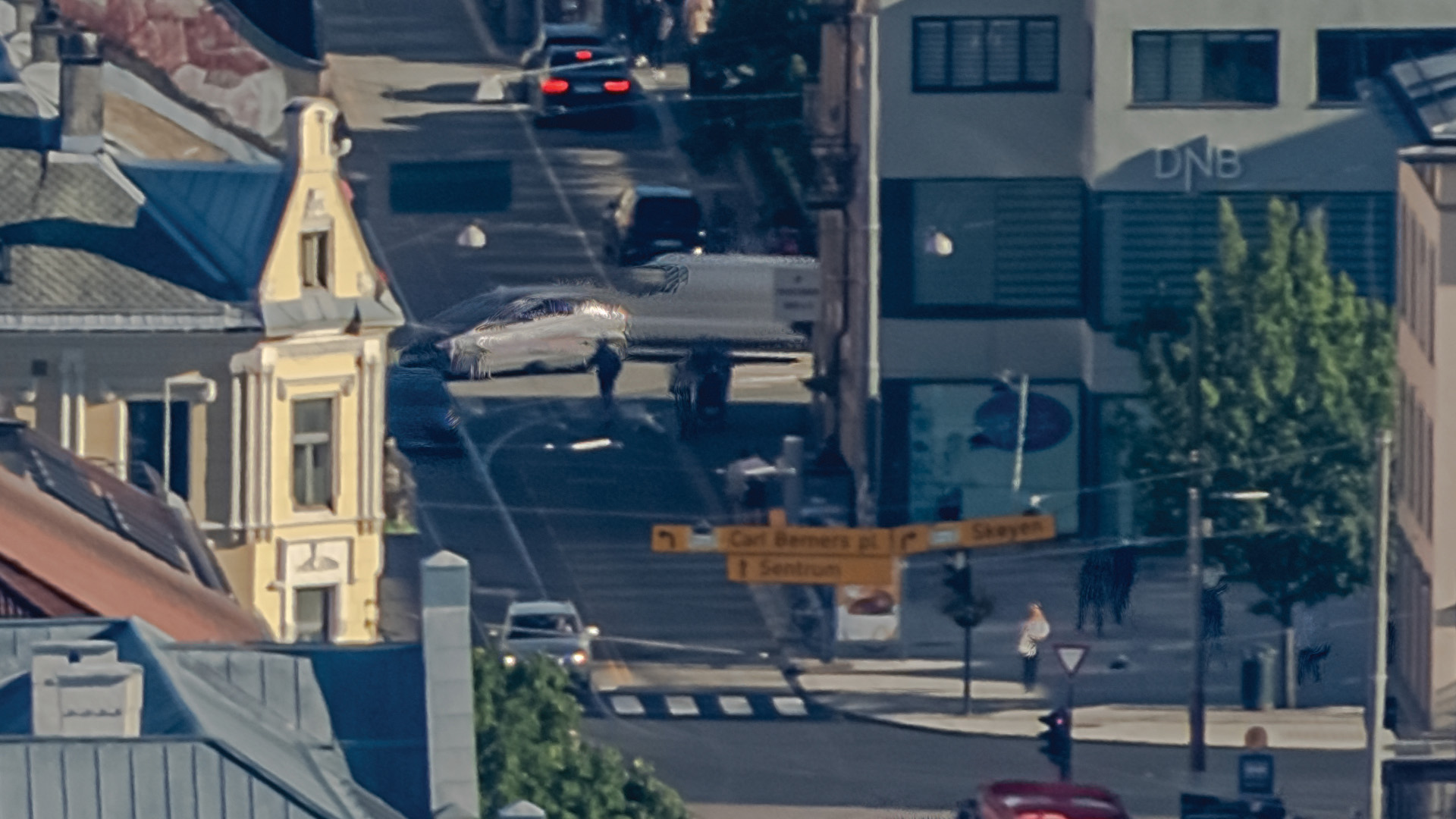
Object within theoretical resolving limits.
The image on left is one single exposure. The image on right is the final image after processing,
upscaling and sharpening. Distance to the signs is about 5 km. Letters in the signs are big enough
for camera to resolve and we see improved image quality. We see generally better quality everywhere in the image, as expected.
4. Shooting the sky
Due to the lack of detail in the sky, photographing it has proven to be the most underestimated challenge of the entire project.
4.1 The problem
All images were shot during 4 days. We had access to the Holmenkollen ski jump only during public opening hours. Shooting the sky on 4 different days on 4 different times of day would not look nice. The sky was shot weeks later on different location with easy access on a day with almost no clouds. It was actually shot twice on different locations, but only images from the second attempt was used. Camera did not have to move and this solved the parallax problem. The few visible clouds could be photographed faster when there was no need to photograph the lower part of the image. Because of the need of faster shooting and minimal need of the higher resolution photographing blue sky, the sky was shot 5 samples pr. image.
Processing the sky proved to be very challenging. The lack of detail made it impossible for the program to determine the correct position of each image. Different approaches were tested by creating XML files to force the images into the right position, but none of these solutions worked. There were also issues with vignetting, which produced visible patterns in the sky. I used software designed for astrophotography to create a precise vignetting profile for my camera and lens combination. However, even this approach was not successful, because vignetting behaves differently depending on how the lens is aligned with the sun, which in some parts of the image is very dominant.
4.1 The solution
The solution was to create a virtual half-dome and place virtual images on it using sine and cosine functions, ensuring that the overlaps matched as closely as possible with the images captured in real world. Each image contained unique patterns to the north, south, east, and west, which corresponded to the patterns in the neighboring images. Once this virtual sky was generated, the stiching software was finally able to process and find a solution for placing every virtual image on the half-dome. There is no way to strech and move the sky to the place which suits you. The moving and streching happens by moving the unique patterns in each image.
Another problem with the sky was that, when completing the full circle of shots several hours later, a visible stitch appeared where the start and end met. Even with a clear blue sky, the blue tone recorded at the beginning was not the same as the one captured by the time the circle was completed. It wasn’t just the brightness that changed, but also the shade of blue. I had to carefully adjust each image to match the exact color of its neighboring frame. Once this was in place, I had to interpolate hundreds of images on the side where the colors were corrected, in order to create a smooth transition toward the stitch area. This was done using a Lua script in Lightroom, which I wrote specifically for the task.
After that, the vignetting issues could be dealt with. The images underwent a complete processing pipeline. They were exported from Lightroom, converted to TIFF, upscaled, stacked, substituted for the virtual versions, rendered, and finally finalized through the generation of an image pyramid with tiles. This procedure involved a considerable amount of data processing and was done several times. This process had to be repeated several times until the visible stich and vignetting was removed.
4.2 Virtual sky images
Example of 2 overlapping virtual sky images. The patterns gave the stiching software a change to find overlapping points. Just before final rendering, the virtual images were replaced by the real sky images and the panorama could be rendered.


5. Rendering and putting it all together
The images were prepared in Lightroom, scaled up by self made software, rendered to 360 panorama and finally converted to multi resolution image pyramid (jpeg).
5.1 Processing
All images were processed by selfmade software using multithreaded producer/consumer architecture. Producer prepared the stack of 16bit tiff images fetched from NFS server and placed the stack in memory queue. When ready, the consumer fetched next stack available and processed the data. Two RTX 4090 GPU cards were organized as virtual resources. Every thread calling CUDA was closely profiled to know exactly how much resources it needed. If not enough resources were available it would go to sleep until some other thread released resources. It would then wake up and ask for the resources again. There were 6 threads of producers and 6 threads of consumers running, each starting it’s own threads to reduce large tasks into smaller tasks requiring smaller amounts of resources. This method balanced the resource very well utilizing both GPU-cards at near full capacity for several weeks. After the images were compiled to 180MP tiff files, final sharpening was added using RawTherapee. Most of the processing was done in 16bit until the part where the images were prepared for stiching. Due to the large amount of data and not much visually gain in processing in 16bit, at this point I switched to 8bit tiff files.
5.2 Stiching
The final result was more than 16.000 x 180MP files imported for stiching. Stiching software has some limitations and is not optimized for panoramas of this size. It struggled with rendering whole panorama as one huge panorama. After giving up the attempts I had to try other approach. The panorama was split into smaller parts, rendered and combined to one huge panorama after rendering. Rendering used 2 week to render the panorama this way. This process was repeated, sometimes in full and other times partly, several times to correct errors, parallax issues and making the sky align with rest of the image.
The panoramas were merged into one large TIFF file (6,145,310,572,420 bytes / 5.58 TB). This file was then split into smaller images for the final adjustments. Since the camera had to be moved to four different positions in the Holmenkollen tower, parallax issues were expected. These issues appeared as poor stitching, with images overlapping in the wrong places. Most of the errors could be corrected in post processing.
5.3 Parallax issues
Since the camera had to be moved on top of the ski tower, there were parallax issues. Parallax issues occur when objects in a scene appear to shift relative to each other between images because the camera was moved to different positions instead of rotating around a single fixed point. When shooting panoramas or 360° images, nearby objects move more noticeably than distant ones if the camera position changes, which leads to alignment conflicts during stitching. This typically happens when the camera is translated rather than only rotated, when it is not rotated around the optical center (also called the entrance pupil), or when images are taken handheld or with an incorrectly adjusted panoramic head. The result is visible stitching errors such as ghosting, duplicated objects, broken straight lines, or tearing in foreground elements. These problems are difficult to fully correct in software because each image represents a different viewpoint, creating geometric inconsistencies that cannot be reconciled across all depths at once. The parallax glitches had to be corrected in Photoshop.
Photoshop can open images up to a maximum size of 300,000 × 300,000 pixels, but for practical reasons the workable limit is 150,000 × 150,000. The huge panorama was therefore split into tiles of this size, and imperfections were corrected.
5.3 Preperations for web
To display a massive gigapixel image online, a technique known as Deep Zoom or image tiling is used. Because a web browser cannot load a multi-gigabyte image all at once, the image is converted into an image pyramid. This process resizes the original image into multiple layers of progressively lower resolution and divides each layer into thousands of small, manageable tiles—typically 512 × 512 pixels.
When a user views the image on a website, a specialized image viewer fetches only the tiles required for the current zoom level and the portion of the image visible on screen. As the user zooms in or pans, low-resolution tiles are seamlessly replaced with higher-resolution ones. This approach provides a fast and smooth viewing experience without requiring the entire image to be downloaded.
The image viewer includes a built-in tool for converting large images into an image pyramid. However, it is not optimized for panoramas of this scale. Converting my panorama using this tool took five days. Because I needed to make numerous small parallax corrections during the process, this was far too slow. To solve this, I developed a high-performance program that generates all pyramid levels in a single pass. This reduced the conversion time to just five hours, significantly improving the overall workflow.
Transferring these massive files between two computers was also time-consuming. Upgrading to a 100 Gbps network provided more bandwidth than I could realistically saturate using file transfers. After upgrading to Windows Server, I was able to use RDMA (Remote Direct Memory Access) for file transfers. This allowed me to achieve sustained transfer speeds of just over 3 GB/s, a substantial improvement over a 10 Gbps network.
After repeating this process many times, I reached a point where I believe the image was ready for public display. For the first time, I could truly see the result of the work invested in this project over the past three years. It has been very interesting journey with many problems which had to be solved. This documents describes the solution used and most of the problems are even not mentioned here.
6. Summary
Creating this panorama has been an interesting journey where I personally discovered several beautiful and unique places in Oslo that I wasn’t even aware of before. Oslo is a beautiful city offering water sports, winter sports, endless forests, lakes, islands, and everything you would expect from a modern urban area. We have culture, entertainment, a clean environment, Nordic architecture, shopping, and the vibrant energy of a contemporary city.
I hope others who share my interest will also enjoy exploring this image and perhaps see Oslo from a new perspective.